The Newton's Force

And .. The World Was Set Into Motion 🏃🏼‍♀️

Act 1: Sir Issac Newton (1687)

The year Galileo departed (January, 1642), almost a year later Newton arrived—January, 1643 [1]. One out, one in; was universe trying some balancing act. Newton, never shy of a good footnote, later remarked that he was "standing on the shoulders of giants" [2]—and yes, Galileo was one of them. So were greats like Al-Baghdadi, Avicenna, Philoponus, Aristotle and others before him. You can see the clear progression of ideas; Newton did not come up with all the ideas in isolation, obviously.

Newton was very unusual and had a very different childhood; it is amazing how these things shape great people [3]. You know, this man once threatened his family that he would burn down the house and kill everyone including his mother and step-father in it.

In 1687, Isaac Newton dropped the Principia Mathematica on the world [4]. His three laws of motion didn’t just change humanity—they promised something wild: the future is predictable.

For the sake of completeness here are the three laws [5]:

First Law (Law of Inertia): An object at rest stays at rest, and an object in motion stays in motion with the same speed and direction unless acted upon by an unbalanced force.
Second Law (Law of Acceleration): The acceleration of an object is proportional to the net force acting on it and inversely proportional to its mass. Mathematically: $F = ma$ .
Third Law (Law of Action and Reaction): For every action, there is an equal and opposite reaction.

Act 2: A step towards deterministic Universe

Newton’s deterministic universe says,

Give me the position and velocity of every particle right now, and I’ll tell you where they’ll be tomorrow, next year, or a thousand years from now.

Suddenly, the world swapped uncertainty for certainty [6]. The uncertainty in the lives of common people was often the core reason why people turned to the powers of Gods, Kings, and Religion. People were not in control of their lives; they barely understood the world and importantly whatever they could understand they could not verify systematically. With more certainty provided by the edict of the Scientific Revolution, people were empowered and the ideas of Gods and religion became less popular (Newton was deeply religious and heretical in nature based on his work [7], what a juxtaposition).

Let's arm ourselves with the certaining provided by Newton's law and try to see what they say about Galileo’s favourite toy: the pendulum. After all, it swings back and forth, keeps time, and looks great in a clock.

Simple Pendulum Diagram

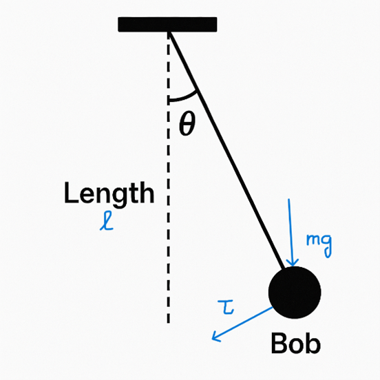
A simple pendulum schematic with length (l) and bob's mass m.

Let's build a simple pendulum: take a ball (the "Bob") of mass $m$ , tie it to a string of length $l$ , and give it a push so it swings at an angle $\Theta$ . Newton's rotational law of motion states [8]:

\vec{\tau} = I \vec{\alpha} \tag{1}

By definition, torque is:

\vec{\tau} = \vec{r} \times \vec{F}_T \tag{2}

Since the tangential force $F_T$ is perpendicular to the position vector $\vec{r}$ (which points along the string), the magnitude becomes:

|\tau| = r F_T \sin(90°) = l \cdot |F_T| \tag{2'}

Gravity provides a force $\vec{F}_g = -mg\hat{j}$ (downward). Decomposing this into radial and tangential components:

Radial component: $F_r = -mg \cos(\Theta)$ (along the string, providing centripetal force)
Tangential component: $F_T = -mg \sin(\Theta)$ (perpendicular to the string, causing rotation)

The tangential component is what creates torque:

F_T = -mg \sin(\Theta) \tag{3}

Substituting equation (3) into equation (2'):

\tau = l \cdot F_T = -lmg \sin(\Theta)

Using equation (1) with $I = ml^2$ and $\alpha = \frac{d^2 \Theta}{dt^2}$ , definition of angular acceleration (twice the derivitive of angular position with time):

-lmg \sin(\Theta) = ml^2 \frac{d^2 \Theta}{dt^2} \tag{4}

Divide both sides by $ml^2$ :

-\frac{g}{l} \sin(\Theta) = \frac{d^2 \Theta}{dt^2}

Rearranging to standard form:

\frac{d^2 \Theta}{dt^2} + \frac{g}{l} \sin(\Theta) = 0 \tag{5}

Equation (5) is the exact equation of motion for the simple pendulum. It is a second-order, nonlinear differential equation that cannot be solved in closed form using elementary functions.

A few other things to note: By "simple pendulum," we mean there is no air resistance (damping) acting on the bob, and no friction at the pivot.

Also, what is a "closed-form" solution? It means a single equation that gives the pendulum's position or velocity at any time (for example, plug in $t = 3$ seconds and get the answer directly). If such an explicit formula exists for a differential equation, we call it a closed-form solution.

Small-Angle Approximation

For small oscillations where $|\Theta| < 0.26$ radians (≈ 15°), we can use the Taylor series approximation [9]. Obviously, this is an engineering approximation; I chose the value arbitrarily thinking it is good enough for the general case. Don't think of this value as a universal truth please. I am an engineer, I am allowed! 🤣😂🤣😂🤣 :

\sin(\Theta) \approx \Theta \tag{6}

Substituting into equation (5):

\frac{d^2 \Theta}{dt^2} + \frac{g}{l} \Theta = 0 \tag{7}

Equation (7) is now linear—the equation for simple harmonic motion. Its general solution is:

\Theta(t) = A \cos(\omega t) + B \sin(\omega t) \tag{8}

where $A$ and $B$ are determined by initial conditions, and the angular frequency is:

\omega = \sqrt{\frac{g}{l}} \tag{9}

The period of oscillation is:

T = \frac{2\pi}{\omega} = 2\pi\sqrt{\frac{l}{g}} \tag{10}

Act 3: An act for people who love mathematics (skip it if you want)

Alert: 🚨 RED-BOX ZONE!

Rigorous Derivation of the General Solution:

Equation (7) is a second-order linear ordinary differential equation. To solve it, we use the characteristic equation method [10]:

\frac{d^2 \Theta}{dt^2} + \frac{g}{l} \Theta = 0

Assume a solution of the form $\Theta(t) = e^{rt}$ , substitute into the equation. Now why in the world you would assume that, it is just a smart mathematcial trick that works and exponential function is easy to work with and we get even more lucky because the function has hidden secret aggrement with circles (this is a deep-hole) to dig right now:

\frac{d^2}{dt^2} e^{rt} + \frac{g}{l} e^{rt} = 0 \implies r^2 e^{rt} + \frac{g}{l} e^{rt} = 0

Divide by $e^{rt}$ (never zero):

r^2 + \frac{g}{l} = 0

Solve for $r$ :

r = 0 \pm i \sqrt{\frac{g}{l}}

r1 = 0 + i \sqrt{\frac{g}{l}}, r2 = 0 - i \sqrt{\frac{g}{l}}

so the general solution can be a linear combination of the two roots, of course assuming linear behavior:

\Theta(t) = C1e^{r1t} + C2e^{r2t}

But what does this mean physically? Let's connect this to real motion. Recall Euler's formula [11]:

e^{i\omega t} = \cos(\omega t) + i\sin(\omega t)

So, for our case $\omega = \sqrt{\frac{g}{l}}$ :

e^{i\sqrt{\frac{g}{l}} t} = \cos\left(\sqrt{\frac{g}{l}} t\right) + i \sin\left(\sqrt{\frac{g}{l}} t\right)

and

e^{-i\sqrt{\frac{g}{l}} t} = \cos\left(\sqrt{\frac{g}{l}} t\right) - i \sin\left(\sqrt{\frac{g}{l}} t\right)

Therefore, any linear combination of $e^{r_1 t}$ and $e^{r_2 t}$ can be rewritten as a linear combination of $\cos$ and $\sin$ functions (using the real and imaginary parts):

\Theta(t) = A \cos\left(\sqrt{\frac{g}{l}}\, t\right) + B \sin\left(\sqrt{\frac{g}{l}}\, t\right)

where $A$ and $B$ are real constants determined by initial conditions. This shows how the exponential solution is equivalent to the familiar oscillatory motion of the pendulum. The general solution is:

\Theta(t) = A \cos\left(\sqrt{\frac{g}{l}}\, t\right) + B \sin\left(\sqrt{\frac{g}{l}}\, t\right)

where $A$ and $B$ are determined by initial conditions. This matches the previous result, but now the derivation is explicit and mathematically rigorous.

Alternatively, the general solution can be written in a single-amplitude, phase-shifted form:

\Theta(t) = C \cos\left(\sqrt{\frac{g}{l}}\, t + \phi\right)

where $C$ (amplitude) and $\phi$ (phase angle) are constants determined by the initial conditions. This form is often convenient for physical interpretation, as it directly encodes the starting displacement and timing of the oscillation.

Special case

Lets assume at t = 0, the pendulum was left at one max end say $\theta = \theta_{max}$ , let us plug these in the last equation, we will have,

\Theta(0) = C \cos\left(0 + \phi\right) = \theta_{max}

Hence, we know that

C = \theta_{max}

also assume the velocity of the pendulum when it was left at extreme point was zero, then we can say,

\Theta^{`}(0) = C \sin\left(0 + \phi\right) = 0

by this we can say that,

\phi = 0

Hence, for the special case, when the "Bob" was left at extreme position at zero velocity the equation of motion of pendulum is simply:

\Theta(t) = \theta_{max} \cos\left(\sqrt{\frac{g}{l}}\, t\right)

Now, what this is a bit too much and we made several approximations in the way, small angle and what not, if we want to simulate any general case, yes even non-linear one, we can use the help of a computer. That's where numerical methods come in. Let us do that later, this is already a lot on the plate for now.

Act 4: Pre-Finale - Explore Newton's Pendulum

Experiment with the pendulum below! Adjust the length, mass, and gravity sliders. Try to match the period you observe with the formula $T = 2\pi\sqrt{\frac{l}{g}}$ . What happens if you set gravity to the Moon’s value? Or make the pendulum very short? It is the same as Galileo's pendulum simulation, but now you can appreciate it more.

Newton’s Pendulum Explorer

Mass: 1.00 kg

Length: 1.50 m

Gravity (g): 9.81 m/s²

Formula: Period T = 2π√(L/g) ≈ 2.457 seconds

Note: Mass does not affect the period in simple pendulum motion (for small angles). Try changing the length to see the period change!

Act 5: Finale - Interactive Exploration: Applying Forces and Observing Acceleration

Now let's explore Newton's Second Law directly! In the widget below, you can apply a force to a ball and watch how it accelerates. The key insight: the acceleration depends on both the force AND the mass.

Try this:

Keep the force constant and increase the mass—notice the ball accelerates slower!
Keep the mass constant and increase the force—the acceleration increases.

This demonstrates the core of Newton's Second Law: a = F/m. A heavier ball resists acceleration more—it has more inertia.

Newton's Second Law: F = ma

Mass: 1.0 kg

Applied Force: 10.0 N

How it works:

Click "Start" to begin the simulation.
Click "Hit Ball →" to apply a force to the red ball.
Red arrow: The force being applied (in Newtons).
Orange arrow: The acceleration caused by the force (in m/s²).
Blue text: The velocity of the ball as it moves.
Try different masses and forces. Remember: a = F/m — heavier balls accelerate less!

References

Westfall, R.S. (1980). Never at Rest: A Biography of Isaac Newton. Cambridge University Press. pp. 53-54. ISBN 978-0-521-27435-7.
Newton, I. (1675). Letter to Robert Hooke, February 5, 1675. "If I have seen further it is by standing on the shoulders of Giants." The Newton Project
Gleick, J. (2003). Isaac Newton. Vintage Books. Chapter 1: "What Manner of Child". ISBN 978-1-4000-3295-2.
Newton, I. (1687). Philosophiæ Naturalis Principia Mathematica. First Edition, London. Digital facsimile at Cambridge Digital Library
Newton, I. (1687). Principia, Book I: "Axioms, or Laws of Motion." Translated by I.B. Cohen & A. Whitman (1999), University of California Press. Archive.org facsimile
Laplace, P.S. (1814). Essai philosophique sur les probabilités. Paris. The classic statement of determinism: "An intellect which at a certain moment would know all forces..." Stanford Encyclopedia: Causal Determinism
Snobelen, S.D. (1999). "Isaac Newton, heretic: the strategies of a Nicodemite." The British Journal for the History of Science, 32(4), pp. 381-419. JSTOR
Goldstein, H., Poole, C., & Safko, J. (2002). Classical Mechanics, 3rd ed. Addison-Wesley. Chapter 1: "Survey of the Elementary Principles." ISBN 978-0-201-65702-9.
Brook Taylor (1715). Methodus Incrementorum Directa et Inversa. London. Original work introducing the Taylor series. Archive.org
Boyce, W.E. & DiPrima, R.C. (2012). Elementary Differential Equations and Boundary Value Problems, 10th ed. Wiley. Chapter 3: "Second Order Linear Equations." ISBN 978-0-470-45831-0.
Euler, L. (1748). Introductio in analysin infinitorum, Vol. 1, Chapter VIII. Lausanne. The formula $e^{ix} = \cos x + i \sin x$ appears here. Euler Archive

The Newton's Force

The Newton's Force

And .. The World Was Set Into Motion 🏃🏼‍♀️

Act 1: Sir Issac Newton (1687)

Act 2: A step towards deterministic Universe

Small-Angle Approximation

Act 3: An act for people who love mathematics (skip it if you want)

Special case

Act 4: Pre-Finale - Explore Newton's Pendulum

Newton’s Pendulum Explorer

Act 5: Finale - Interactive Exploration: Applying Forces and Observing Acceleration

Newton's Second Law: F = ma

Newton’s Force Quiz

References